
Please note that this tutorial (including the formatting) is a work in progress. I’m simply posting my progress in good faith. Your comments are welcomed.
Introduction
The news of Parsey McParseface achieving record-breaking parsing accuracy was interesting and thought-provoking. As far as I remember, it even hit some major public news outlets. Running the example parser and seeing English sentences magically get parsed might have made you wonder what the significance and implication of this accomplishment is and how it actually works. If you’re like me, reading the SyntaxNet page, as full as it is with beautiful diagrams and claims of novel architecture, raised more questions than answers. While it does a decent job explaining the overview (especially of the improved parts compared to previous work), it stops short of providing any real specification for the data structures or vectors passing through the system. It is a beautiful model that you can’t fully appreciate unless you understand the inner workings. And to do that, you’d typically need to look at a lot of prior work on the manner.
This tutorial is meant to explain SyntaxNet to programmers with interest in understanding dependency parsers but with little background in ProtoBuf, bazel, TensorFlow, CoNLL, arc-standard parsers, and most of all, math. It would be wrong to say that documentation doesn’t exist, but I’ve found that the best documentation for SyntaxNet is the source code itself. I’ve tried to outline some of the things I’ve learned while analyzing the SyntaxNet source code. As far as I know, most of this should apply to the POS tagging portion of SyntaxNet as well. (By the way, I haven’t finished understanding everything, either.)
Overview
POS tagging and dependency parser training is possible with a unified transition-system based architecture. Inputs are features of parser states, and the output is the next parser action to take based on the knowledge available from features. For the tagger, the action will simply be the POS tag to choose, and for dependency parsing, the arc-standard transition to take.
At first, a greedy parser is “pretrained”. And, then a beam parser uses a “structured graph builder” to “fix” the wrong decisions of the greedy parser when it realizes that a certain transition sequence has “gone off the golden path”.
With a good set of features, greedy parsers are still very powerful. To be honest, beam search offers less than 1% performance improvement on POS tagging for English, and around 2% on dependency parsing. (Andor et al., 2016) However, it’s worth mentioning that beam search and so-called semi-supervised techniques known as “Tri-Training” (in which a corpus is augmented when the result of two independent parsers matches) can improve accuracy marginally. I will only be covering the greedy parser portion (because I have yet to understand the inner workings of beam search).
Let’s look at what happens during the training process.
-
- Lexicon computation (LexiconBuilder Op)
Walks through the input corpus
Calculates frequency of words, characters, POS tags, DEPREL labels, etc.
Generates label-map, prefix-table, tag-to-category files (explained later) - FeatureSize Op
Determines size of features and domain of possible feature values, along with embedding dimensions and number of actions - Well-formed filtering of training set (WellFormedFilter Op)
Optional - Projectivization of training set (ProjectivizeFilter Op)
Optional, but can projectivize a non-projective corpus “Lift the shortest non-projective arc until the document is projective”
Projectivized corpus means that the arc-standard transition system can be used - Build greedy parser graph
- Add training corpus
Utilize GoldParseReader Op to derive “gold actions” for the input corpus
Build trainer to minimize cost of network output (minimizing their difference from these “gold actions”)
- Add evaluation step against testing corpus
Uses DecodedParseReader Op to run network
- Perform epoch-based model training
- Lexicon computation (LexiconBuilder Op)
Now, we’ll look more into details. The tutorial will now quickly take on a much more programming-oriented tone.
ProtoBuf Structures
These are structures that are often passed between Python and C++ or serialized.
Sentence (ABI definition: sentence.proto)
Represents a block of CoNLL-U (which should be a sentence).
docid: Arbitrary identifier for document [filename + ‘:’ + sentence_count?] (proto_io.h:167)
text: Simply token words (FORM CoNLL-U column) joined by a space [“ “] (text_formats.cc:135)
start,end of the token refers to starting and ending string indices of that token as it corresponds to the sentence text
token[]: Tokenization of the sentence
Token (ABI definition: sentence.proto)
Represents one line of CoNLL-U. (text_formats.cc:125)
| Property | CoNLL-U Column |
| (array index) | ID-1 if no multi-word tokens
multi-word tokens are skipped (text_formats.cc:106). Unclear if proper operation is possible with multi-word tokens |
| word | FORM |
| (unused) | LEMMA |
| category (category POS tag) | UPOSTAG (or empty if JoinCategoryToPos() is used) |
| tag | XPOSTAG (and if requested, UPOSTAG may be prepended like UPOSTAG ’++’ XPOSTAG [JoinCategoryToPos()]) |
| TokenMorphology attributes | FEATS (and if requested, XPOSTAG [AddPosAsAttribute()])
a1=v1|a2=v2|… or v1|v2|… |
| head (-1 for root, 0 for first element, …) | HEAD (0 for root, 1 for first element, …) |
| label | DEPREL |
| (unused) | DEPS |
| (unused) | MISC |
start,end,break_level are additional properties of a token.
start,end are used for character index within space-joined words for sentence
break_level is used to determine how the current token was separated from previous token
TokenMorphology (ABI definition: sentence.proto)
Attribute
{
name: string name of morphology feature
value: string value of morphology feature
}
attribute[]: array of Attributes representing all morphology features
SparseFeatures (ABI definition: sparse.proto)
id[]: uint64 array of feature values
weight[]: floating point array of feature weights (1.0 unless otherwise specified)
description[]: string translation array of feature values (not always used)
All arrays have the same number of elements.
AffixTableEntry (ABI definition: dictionary.proto)
AffixEntry
{
form: affix as a string
length: length of affix in UTF-8 characters
shorter_id: the id of the ancestor affix that is one character shorter, or -1 none exists (used for lookup optimization)
}
type: type of affix table (prefix or suffix), string
max_length: max length of prefix or suffix in the table
affix[]: array of AffixEntry structures, in order of affix ID
TokenEmbedding (ABI definition: dictionary.proto)
token: UTF-8 bytes? of token word
count: frequency that this word occurred in the training corpus
Vector
{
values[]: array representing word embedding vector
}
vector: word vector for respective token (Vector)
C++ Structures
These are structures used in the C++ code.
Maps
TermFrequencyMap
- Map between term (label or POS tag) and frequency
- Sorted by descending order of frequency, and lexicographically on term (term_frequency_map.cc)
- Terms must be all unique (no duplicates, obviously)
- Terms that are too low or high in frequency can be excluded
TagToCategoryMap
- Map between XPOSTAG(tag) and UPOSTAG(category) (fine to coarse POS tags)
- N to 1 mapping: one tag cannot be mapped to more than one category
Tables
AffixTable
- Two table types: Prefix/Suffix
- An affix represents a prefix or suffix of a word of a certain length.
- Each affix has a unique id and a textual form.
- An affix also has a pointer to the affix that is one character shorter. This creates a chain of affixes that are successively shorter.
- Affixes are hashed (on their terms) into buckets (hash table)
There are other structures not covered here.
LexiconBuilder
This task collects term statistics over a corpus and saves a set of term maps. It computes the following:
-
- TermFrequencyMap words
- Frequency map of all words (CoNLL-U FORM)
- Includes punctuation
- TermFrequencyMap lcwords
- Frequency map of lower case words
- Includes punctuation (according to source code)
- TermFrequencyMap tags
- Frequency map of fine POS tags (XPOSTAG)
- TermFrequencyMap categories
- Frequency map of coarse POS tags (UPOSTAG)
- TermFrequencyMap labels
- Frequency map of DEPREL
- TermFrequencyMap chars
- Frequency map of individual characters
- AffixTable prefixes(AffixTable::PREFIX, max_prefix_length_)
- lexicon_max_prefix_length: default 3
- AffixTable suffixes(AffixTable::SUFFIX, max_suffix_length_)
- lexicon_max_suffix_length: default 3
- TagToCategoryMap tag_to_category
- Map fine POS tags to coarse POS categories
- TermFrequencyMap words
Task Context Files
(lexicon_builder.cc: ~138)
The filenames for these maps and tables must be specified in context.pbtxt in the input clauses. But the reality is that these aren’t necessarily input in the sense that they need to be generated by the user. SyntaxNet is the one that generates them and uses them for future tasks.
It’s unclear which ones are optional.
Calculated during lexicon builder:
- word-map: TermFrequencyMap for FORM (words)
- lcword-map: TermFrequencyMap for lowercase version of FORM (words)
- tag-map: TermFrequencyMap for POS tags of tokens (see Token section)
- category-map: TermFrequencyMap for categories themselves (UPOSTAG if used, see Token section)
- label-map: TermFrequencyMap for DEPREL labels
- char-map: TermFrequencyMap for individual characters in FORM (words)
- prefix-table: AffixTable for word prefixes of specified length
- Stored in ‘recordio’ format (protocol: AffixTableEntry dictionary.proto)
- suffix-table: AffixTable for word suffixes of specified length
- Stored in ‘recordio’ format (protocol: AffixTableEntry dictionary.proto)
- tag-to-category: TagToCategoryMap for <XPOSTAG, UPOSTAG>
Not calculated during lexicon builder:
- char-ngram-map
- character ngrams of length 3 default (max_char_ngram_length, class CharNgram)
- TODO: how is this used?
- morph-label-set
- ?
- morphology-map
- ?
File Formats
Name is the option key looked up in context.pbtxt to find filename to load. It’s the type of file. When executing parser_trainer you can actually specify the context name indicators for the files needed for input, so the name is actually up to you. Here we’ll list the typical names used for each respective file.
Some formats use ProtoBuf, and header files are generated dynamically during the compile process to read in these structures. The last column indicates whether or not the file is generated by SyntaxNet itself or required by SyntaxNet initially as input.
| Name | File Format | Record Format | System Generated? |
| stdin-conll stdout-conll |
(stdin) (stdout) |
conll-sentence (CoNLL-U) | No Yes |
| training-corpus
tuning-corpus |
text | conll-sentence (CoNLL-U) | No No |
| morph-label-set | recordio | token-morphology
Uses TokenMorphology structure |
Yes |
| prefix-table suffix-table |
recordio | affix-table AffixTable::Read() Uses AffixTableEntry structure |
Yes Yes |
| (other -map files and tag-to-category) | text | (plain text) | Yes |
| word-embeddings (not often used) | recordio | WordEmbeddingInitializer::Compute()
TokenEmbedding protocol defined in dictionary.proto See https://github.com/tensorflow/models/issues/102 |
No |
Formats
- recordio:
- TensorFlow binary format (TFRecordWriter)
- Used mainly for storing maps, tables, and vectors, including word embeddings
- See https://github.com/tensorflow/models/issues/102
- text:
- UTF-8
- Parsed by individual classes themselves
Feature Extraction System
Primary Feature Types
TermFrequencyMapFeature (sentence_features.h)
- Uses a TermFrequencyMap to store a string->int mapping
- Uses index of term in file (first mapping would be index 0)
- Terms are sorted in descending frequency, so that would mean index 0 would be the most frequent term
TermFrequencyMapSetFeature
- Specialization of TokenLookupSetFeature
- Maps a set of values to a set of term indices (rather than just one value) for each token
- Each value in the set is a term index discovered by LookupIndex()
LexicalCategoryFeature
- Returns an index (representing a small, predefined category) describing the input lexicon (e.g., whether the token has hyphens, how it’s capitalized, etc)
- In sentence_features.h, ‘cardinality’ means number of possible categories
AffixTableFeature
- Returns the Affix ID of a fixed-length prefix or suffix on a token or an unknown value of affix table size if it’s not found
- ID must be unique
- (ID does not appear to have any special sort order?)
- Unknown Value specifies which value is used when the lookup fails
- Usually this is the size of the term array, which would be a reserved index because it wouldn’t exist (valid indices: 0-term_map.size()-1)
Usable Token Features
| Feature | Storage Method | Unknown Value | ||||||||||
| Word | TermFrequencyMapFeature(“word-map”) Looks up term index of token.word() [FORM] |
term_map().size() | ||||||||||
| Char | TermFrequencyMapFeature(“char-map”) Looks up term index of token.word()??? Perhaps this only works with tokens whose words happen to be single characters |
term_map().size()+1
(break chars/whitespace is term_map().size()) |
||||||||||
| LowercaseWord | TermFrequencyMapFeature(“lc-word-map”) Looks up term index of lowercased token.word() [FORM] |
term_map().size() | ||||||||||
| Tag | TermFrequencyMapFeature(“tag-map”) Looks up term index of token.tag() |
term_map().size() | ||||||||||
| Label | TermFrequencyMapFeature(“label-map”) Looks up term index of token.label() |
term_map().size() | ||||||||||
| Hyphen | LexicalCategoryFeature(“hyphen”) Whether word has hyphen or not
|
N/A? | ||||||||||
| Capitalization | LexicalCategoryFeature(“capitalization”) Describes how word is capitalized
|
N/A? | ||||||||||
| PunctuationAmount | LexicalCategoryFeature(“punctuation-amount”) Describes the amount of punctuation in the word
|
N/A? | ||||||||||
| Quote | LexicalCategoryFeature(“quote”) Describes whether the word is an open or closed quotation mark. Only applicable if word is “, ”, or one letter long and a quote.
[is_open_quote/is_close_quote()]: see char_properties.h for all quote types |
N/A? | ||||||||||
| Digit | LexicalCategoryFeature(“digit”)
Describes the amount of digits in the word
|
N/A? | ||||||||||
| Prefix | AffixTableFeature(AffixTable::PREFIX) Looks up Affix ID of particular prefix ID must be unique |
affix_table_->size() | ||||||||||
| Suffix | AffixTableFeature(AffixTable::SUFFIX)
Looks up Affix ID of particular suffix |
affix_table_->size() | ||||||||||
| CharNgram | TermFrequencyMapSetFeature(“char-ngram-map”) Looks up term indices of n-grams (of [1,max_char_ngram_length]) within string pieces of a token[CharNgram::GetTokenIndices()] (sentence_features.cc) |
term_map().size() | ||||||||||
| MorphologySet | TermFrequencyMapSetFeature(“morphology-map”)
Looks up term indices of each attr=value pair from token’s morpohlogy extended attribute [MorphologySet::GetTokenIndices()] (sentence_features.cc) |
term_map().size() |
Feature Embedding System
This section describes how the features extracted are actually embedded and wrapped for use in embedding-based models such as neural networks. We will follow sentences and tokens as they flow through the various components of the system.
Features are grouped into blocks that share an embedding matrix and are concatenated together. These are defined in context.pbtxt. Semicolons (;) determine the feature groups. This is extremely subtle. These feature descriptions are called “embedding FML”, perhaps short for feature markup language. The number of feature groups is equal to the number of FML text split by semicolons.
When the FML is parsed, a feature extractor is created for each feature group. Then, for each feature within the feature group, a feature function descriptor is created. The feature function descriptors are stored under each feature extractor.
By the way, in context.pbtxt, parameters starting with brain_tagger_ are used for the POS tagger and those with brain_parser_ are used to configure the dependency parser component of SyntaxNet. However, these prefixes can be changed using the –arg_prefix parameter to parser_trainer.
It’s important to realize that input features are determined in the context of a particular parser state, not necessarily a particular token. The new input token being processed is just one part of the parser state. Any particular token’s features will almost always be used more than once! This is because the same token can end up on the stack again, depending on the type of transition we do. Most member variables in the ParserState class are fair-game for input features. Input parser states are mapped to output parser states. It’s just one ParserState to another ParserState. Output parser states represent the best next parser action for a particular input state. This makes the model very simple in principle.
Basic Structures
FeatureType represents a feature itself (input.tag, stack.child(-1).sibling(1).label, etc..)
FeatureValue is simply an int64.
FloatFeatureValue: FeatureValue(int64) is mapped to <uint32, float32> in memory using a union
FeatureVector stores <FeatureType, FeatureValue> pairs.
Here is an example of a definition of feature groups for a dependency parser from context.pbtxt:
Parameter {
  name: 'brain_parser_embedding_dims'
  value: '8;8;8'
}
Parameter {
  name: 'brain_parser_features'
  value: 'input.token.word input(1).token.word input(2).token.word stack.token.word stack(1).token.word stack(2).token.word;input.tag input(1).tag input(2).tag stack.tag stack(1).tag stack(2).tag;stack.child(1).label stack.child(1).sibling(-1).label stack.child(-1).label stack.child(-1).sibling(1).label'
}
Parameter {
  name: 'brain_parser_embedding_names'
  value: 'words;tags;labels'
}
An alternate representation of this is the following table:
| Feature Group | Embedding Name | Embedding Dimension |
| input.token.word input(1).token.word input(2).token.word stack.token.word stack(1).token.word stack(2).token.word |
words | 8 |
| input.tag input(1).tag input(2).tag stack.tag stack(1).tag stack(2).tag |
tags | 8 |
| stack.child(1).label stack.child(1).sibling(-1).label stack.child(-1).label stack.child(-1).sibling(1).label |
labels | 8 |
The embedding name is not important. It can be anything arbitrary. However, grouping features of the same type together seems to be a good idea. Otherwise, all values from both features would have to be embedded into the same vector, and for some reason this might not work well.
Feature group specifies the features that should be concatenated with each other when going into the input layer.
Embedding dimension is something we will look at more in depth later. Basically, embeddings for any given group become a tensor of shape (NumFeatureIDs, EmbeddingDim), where NumFeatureIDs is the total number of unique feature values possible for all feature types within that feature group.
In order to begin embedding input and output features, we have to determine several things. These calculations are performed by the FeatureSize Op in lexicon_builder.cc.
Input Features
- Feature size
- The number of features within a group (easy to see from context.pbtxt)
- Domain size
- The maximum of the number of possible values for all given features in the group [largest domain size of any individual feature type]
- Embedding dimensions
- embedding_dims for the group (again, simply read from context.pbtxt)
Output Features
We also need to embed the output parser actions to take. For the tagger we need to embed the POS tags, and for the dependency parser we need to embed the output arc-standard transitions. For that, we only need to determine the number of possible actions to take at any particular parser state. This is the only output feature. And to my knowledge, this is the only feature encoded as a one-hot vector in the neural network. It’s encoded as a one-hot vector so that the softmax activation function can be used to determine a probability for each transition action.
The number of actions for the POS tagger is defined as the number of tags.
The number of actions for the dependency parser is defined as T*2+1, where T is the number of DEPREL labels. LEFT-ARC(T), RIGHT-ARC(T), SHIFT MUST be defined. All actions are encoded into a single integer using bitshifting/bitmasking. See arc_standard_transitions.cc:
// The transition system operates with parser actions encoded as integers:
//  - A SHIFT action is encoded as 0.
//  - A LEFT_ARC action is encoded as an odd number starting from 1.
//  - A RIGHT_ARC action is encoded as an even number starting from 2.
Training feature extraction
SentenceBatch reads in slots of up to max_batch_size sentences at once and stores a ParserState object for each slot. As training proceeds, each sentence slot’s token is advanced (index incremented). Once the end token is reached for a slot, a new sentence is read for that slot. During this process, features are extracted for each input parser state and each parser state for each sentence is advanced based on the gold parser (for training).
Order of Execution
Don’t look at this as an execution stack exactly, but to provide some context, here is the order in which the following operations are executed and their purpose specified in the second column.
(top: executed first)
| Function | Task |
| ParsingReader::Compute | Iterates over training sentence batches |
| EmbeddingFeatureExtractor::ExtractSparseFeatures | Extracts requested features from a particular parser state |
| for (i = 0; i < featureGroupCount; i++) FeatureExtractor[i]::ExtractFeatures |
Each FeatureExtractor extracts all features of a certain feature group from a particular parser state. Each group will eventually extract one FeatureVector. |
| for (k = 0; k < FeatureExtractor[i].featureFunctionCount; k++)
FeatureExtractor[i]::functions[k]::Evaluate |
Each FeatureFunction of each FeatureExtractor extracts its respective feature. In other words, each feature within a group extracts what it needs from the specified parser state. |
| GenericEmbeddingFeatureExtractor::ConvertExample | Operates over all features extracted from all feature groups.
Converts vector of FeatureVector objects to vectors of vectors of SparseFeatures objects, defined in sparse.proto |
We’ve introduced a lot of information. So it’s probably better that we look at an example before going further.
Case Study
To see how everything actually works, we will use the parser_trainer_test test suite with some modified SyntaxNet code for adding logs. This uses the task context in testdata/context.pbtxt and training data testdata/mini-training-set.
To run a test and see all print statements, use the following (from syntaxnet/syntaxnet directory):
bazel test --test_output=all //syntaxnet:parser_trainer_test
Note that you won’t see the same output as I provide here because I have deliberately added more logging to the source code. And, if you understand SyntaxNet from this tutorial, you hopefully won’t need to be adding logging.
FeatureSize::Compute Op
This is the Op that computes feature sizes. Let’s see what happens when we use the embedding_names and embedding_dims defined in the test context:
brain_parser_embedding_dims: '8;8;8'
brain_parser_embedding_names: 'words;tags;labels'
The features we will be using are as follows (again, semicolons delimit feature groups):
'input.token.word input(1).token.word input(2).token.word stack.token.word stack(1).token.word stack(2).token.word;input.tag input(1).tag input(2).tag stack.tag stack(1).tag stack(2).tag;stack.child(1).label stack.child(1).sibling(-1).label stack.child(-1).label stack.child(-1).sibling(1).label'
As you can probably figure out this means we will have three groups of features. Yes, this corresponds with the number of semicolon-separated elements in the embedding_dims and embedding_names! That means that each feature group has a dimension and name, and all group definitions are delimited by semicolons. Again, embedding_names is completely arbitrary.
Next, let’s see how this FeatureSize operation works its magic. To do that, let’s look a little more in-depth at how feature values are actually stored. Let’s look at the map file that handles token.word in testdata/ (this is generated by the parser trainer during lexicon computation).
Loaded 547 terms from /tmp/syntaxnet-output/word-map.
I ./syntaxnet/feature_types.h:86] ResourceBasedFeatureType(0x7fcbe810cda0): ctor(input.token.word, resource base values count=548, special values count: 1)
Values count include terms count plus a NULL/UNKNOWN reserved value.
I ./syntaxnet/feature_types.h:92] ...Resource(0x7fcbe8001f70)[44]: 99-year-old
...
I ./syntaxnet/feature_types.h:92] ...Resource(0x7fcbe8001f70)[547]: <UNKNOWN>
(token.word: total of 547 term values plus <UNKNOWN> and <OUTSIDE> = 549)
These indices correspond with all possible token.word values! If we look at word-map, the index of the array will be the 1-based line number in the file minus 2. That’s because the first line of word-map has the number of words, and the Resource class uses a 0-based index to store its terms. The <UNKNOWN> value is not encoded in word-map and is instead added at the very end as a reserve value. Remember, that these word tokens (except the non-term values of course) are stored in descending frequency that they occur in the corpus (that is, the input sentences). So, index 0 represents the most frequent term.
This happens the exactly same way for token.tag and tag-map.
...
I ./syntaxnet/feature_types.h:92] ...Resource(0x7fcbe8003278)[13]: VBZ
(token.tag: total of 36 term values plus <UNKNOWN> and <OUTSIDE> and <ROOT> = 39)
And token.label:
...
I ./syntaxnet/feature_types.h:92] ...Resource(0x7fcbe8004668)[18]: nsubjpass
(token.label: total of 39 term values plus <UNKNOWN> and <OUTSIDE> and <ROOT> = 42)
NOTE: tags and labels also add a <ROOT> value during runtime via the RootFeatureType class. <OUTSIDE> represents values outside of the stack or input that cannot be reached (we can’t reference the previous token when we’re on the first token, for example). <UNKNOWN> seems to be used internally for some other case.
This may be described more in detail here: http://www.petrovi.de/data/acl15.pdf
FeatureSize Op Return Value
After all the features are analyzed, the FeatureSize Op returns the following for each feature group:
I syntaxnet/lexicon_builder.cc:232] FeatureSize[0]=6
I syntaxnet/lexicon_builder.cc:234] DomainSize[0]=549
I syntaxnet/lexicon_builder.cc:236] EmbeddingDims[0]=8
I syntaxnet/lexicon_builder.cc:232] FeatureSize[1]=6
I syntaxnet/lexicon_builder.cc:234] DomainSize[1]=39
I syntaxnet/lexicon_builder.cc:236] EmbeddingDims[1]=8
I syntaxnet/lexicon_builder.cc:232] FeatureSize[2]=4
I syntaxnet/lexicon_builder.cc:234] DomainSize[2]=42
I syntaxnet/lexicon_builder.cc:236] EmbeddingDims[2]=8
I syntaxnet/lexicon_builder.cc:248] TransitionSystem_NumActions=79
TransitionSystem_NumActions is defined as T*2+1, where T is the number of DEPREL labels. LEFT-ARC(T), RIGHT-ARC(T), SHIFT MUST be defined. So in this case, 39*2+1=79 possible actions. All actions are encoded into a single integer using bitshifting/bitmasking. See arc_standard_transitions.cc.
Parsing Features
If we look at the first entry in testdata/mini-training-set:
1	I	_	PRP	PRP	_	2	nsubj	_	_
2	knew	_	VBD	VBD	_	0	ROOT	_	_
3	I	_	PRP	PRP	_	5	nsubj	_	_
4	could	_	MD	MD	_	5	aux	_	_
5	do	_	VB	VB	_	2	ccomp	_	_
6	it	_	PRP	PRP	_	5	dobj	_	_
7	properly	_	RB	RB	_	5	advmod	_	_
8	if	_	IN	IN	_	9	mark	_	_
9	given	_	VBN	VBN	_	5	advcl	_	_
10	the	_	DT	DT	_	12	det	_	_
11	right	_	JJ	JJ	_	12	amod	_	_
12	kind	_	NN	NN	_	9	dobj	_	_
13	of	_	IN	IN	_	12	prep	_	_
14	support	_	NN	NN	_	13	pobj	_	_
15	.	_	.	.	_	2	punct	_	_
We can walk through how exactly the features are processed.
Tag(0x35f57a8): ComputeValue(token=0x7f7da40018d0, token.tag()=PRP): result value(int64)=10
Tag(0x35f57a8): ComputeValue(token=0x7f7da4001600, token.tag()=VBD): result value(int64)=8
Tag(0x35f57a8): ComputeValue(token=0x7f7da4002110, token.tag()=PRP): result value(int64)=10
Tag(0x35f57a8): ComputeValue(token=0x7f7da4001c20, token.tag()=MD): result value(int64)=20
Tag(0x35f57a8): ComputeValue(token=0x7f7da40021a0, token.tag()=VB): result value(int64)=11
Tag(0x35f57a8): ComputeValue(token=0x7f7da4002280, token.tag()=PRP): result value(int64)=10
Tag(0x35f57a8): ComputeValue(token=0x7f7da4001fe0, token.tag()=RB): result value(int64)=9
Tag(0x35f57a8): ComputeValue(token=0x7f7da40026e0, token.tag()=IN): result value(int64)=3
Tag(0x35f57a8): ComputeValue(token=0x7f7da4002ae0, token.tag()=VBN): result value(int64)=12
Tag(0x35f57a8): ComputeValue(token=0x7f7da4001ac0, token.tag()=DT): result value(int64)=2
Tag(0x35f57a8): ComputeValue(token=0x7f7da4001b50, token.tag()=JJ): result value(int64)=4
Tag(0x35f57a8): ComputeValue(token=0x7f7da4002810, token.tag()=NN): result value(int64)=0
Tag(0x35f57a8): ComputeValue(token=0x7f7da40023e0, token.tag()=IN): result value(int64)=3
Tag(0x35f57a8): ComputeValue(token=0x7f7da4002c00, token.tag()=NN): result value(int64)=0
Tag(0x35f57a8): ComputeValue(token=0x7f7da4002ce0, token.tag()=.): result value(int64)=5
Note again that the integer lookup value of the tag is based on the order of that tag in the tag-map file, which is based on descending frequency of occurrence in corpus.
Sparse->Deep Embedding Process
Now, it’s time to see how these feature values actually get embedded. Although they will all eventually be converted to dense embeddings (not one-hot encodings), first, let’s look at their sparse representation.
When features were added to FeatureVectors, they are stored at different data offsets within the group. The following is an example using the first sentence and first token of the test corpus, the CoNLL-U of which was mentioned above.
Sparse Representations
Feature Group[0]: ‘words’ (6 features total)
| Feature Type | Name Value | Integer Value | Storage Offset |
| input.token.word | I | 50 | 0 |
| input(1).token.word | knew | 372 | 1 |
| input(2).token.word | I | 50 | 2 |
| *stack.token.word | <OUTSIDE> | 548 | 3 |
| *stack(1).token.word | <OUTSIDE> | 548 | 4 |
| *stack(2).token.word | <OUTSIDE> | 548 | 5 |
- <OUTSIDE> means there is nothing on the stack, and therefore the feature value is encoded as the reserved <OUTSIDE> term
Feature Group[1]: ‘tags’ (6 features total)
| Feature Type | Name Value | Integer Value | Storage Offset |
| input.tag | PRP | 10 | 0 |
| input(1).tag | VBD | 8 | 1 |
| input(2).tag | PRP | 10 | 2 |
| stack.tag | <ROOT> | 38 | 3 |
| *stack(1).tag | <OUTSIDE> | 37 | 4 |
| *stack(2).tag | <OUTSIDE> | 37 | 5 |
Feature Group[2]: ‘labels’ (4 features total)
| Feature Type | Name Value | Integer Value | Storage Offset |
| stack.child(1).label | <ROOT> | 41 | 0 |
| stack.child(1).sibling(-1).label | <ROOT> | 41 | 1 |
| *stack.child(-1).label | <OUTSIDE> | 40 | 2 |
| *stack.child(-1).sibling(1).label | <OUTSIDE> | 40 | 3 |
We going to be analyzing an important piece of the SyntaxNet code in the Python side.
Let’s take a look at graph_builder.py:45
def EmbeddingLookupFeatures(params, sparse_features, allow_weights):
 """Computes embeddings for each entry of sparse features sparse_features.


 Args:
   params: list of 2D tensors containing vector embeddings
   sparse_features: 1D tensor of strings. Each entry is a string encoding of
     dist_belief.SparseFeatures, and represents a variable length list of
     feature ids, and optionally, corresponding weights values.
   allow_weights: boolean to control whether the weights returned from the
     SparseFeatures are used to multiply the embeddings.


 Returns:
   A tensor representing the combined embeddings for the sparse features.
   For each entry s in sparse_features, the function looks up the embeddings
   for each id and sums them into a single tensor weighing them by the
   weight of each id. It returns a tensor with each entry of sparse_features
   replaced by this combined embedding.
 """
 if not isinstance(params, list):
   params = [params]
 # Lookup embeddings.
 sparse_features = tf.convert_to_tensor(sparse_features)
 indices, ids, weights = gen_parser_ops.unpack_sparse_features(sparse_features)
 embeddings = tf.nn.embedding_lookup(params, ids)


 if allow_weights:
   # Multiply by weights, reshaping to allow broadcast.
   broadcast_weights_shape = tf.concat(0, [tf.shape(weights), [1]])
   embeddings *= tf.reshape(weights, broadcast_weights_shape)


 # Sum embeddings by index.
 return tf.unsorted_segment_sum(embeddings, indices, tf.size(sparse_features))
params supplies feature embeddings. We will take a look at these later. For Feature Group[2], params would be shape (42, 8). It has one 8-dimensional embedding per possible feature value.
ids stores IDs (index) of all feature values for a token (just 0 to the number of feature values-1). Shape would be (128, ) for Feature Group[2].
indices stores the index of the element used. Shape is always same as ids, (128, ) for Feature Group[2]. This is only significant if an element has multiple feature values. But in our case, there is only one feature value per element.
In UnpackSparseFeatures::Compute we can also see the loop that generates this information received by Python.
for (int64 i = 0; i < n; ++i) {
   for (int j = 0; j < num_ids[i]; ++j) {
     indices(c) = i;
     ids(c) = id_and_weight[c].first;
     weights(c) = id_and_weight[c].second;
     ++c;
   }
 }
We have already analyzed the first token of the first sentence. Because we use sentence batches, the next processed token will be the first token of the second sentence (“The journey through deserts and mountains can take a month.”)
1	The	_	DT	DT	_	2	det	_	_
2	journey	_	NN	NN	_	8	nsubj	_	_
3	through	_	IN	IN	_	2	prep	_	_
4	deserts	_	NNS	NNS	_	3	pobj	_	_
5	and	_	CC	CC	_	4	cc	_	_
6	mountains	_	NNS	NNS	_	4	conj	_	_
7	can	_	MD	MD	_	8	aux	_	_
8	take	_	VB	VB	_	0	ROOT	_	_
9	a	_	DT	DT	_	10	det	_	_
10	month	_	NN	NN	_	8	tmod	_	_
11	.	_	.	.	_	8	punct	_	_
The feature values are therefore as follows:
[“The”, “journey”, “through”, “<OUTSIDE>”, “<OUTSIDE>”, “<OUTSIDE>”]
Feature Group[0]: [11, 369, 509, 548, 548, 548]
[“DT”, “NN”, “IN”, “<ROOT>”, “<OUTSIDE>”, “<OUTSIDE>”]
Feature Group[1]: [2, 0, 3, 38, 37, 37]
[“<ROOT>”, “<ROOT>”, “<OUTSIDE>”, “<OUTSIDE>”]
Feature Group[2]: [41, 41, 40, 40]
For the example, our batch_size is 32.
So that means we will have:
Feature Group[0]: 32 tokens*6 features = 192 elements per batch
Feature Group[1]: 32 tokens*6 features = 192 elements per batch
Feature Group[2]: 32 tokens*4 features = 128 elements per batch
Token feature values are simply concatenated.
indices, ids, weights will all be a vector of the same dimension per group (192, or 128).
Dense Representations
Below are the actual ids passed through SyntaxNet for the first batch.
Key:
Red: sentence 1’s first token features for respective feature group (see earlier in this section for values)
Blue: sentence 2’s first token features for respective feature group
Feature Group[0]
ids[192]: [50 372 50 548 548 548 11 369 509 548 548 548 225 83 93 548 548 548 126 80 265 548 548 548 146 453 39 548 548 548 181 475 247 548 548 548 108 3 143 548 548 548 117 94 377 548 548 548 127 89 25 548 548 548 208 462 217 548 548 548 154 197 1 548 548 548 11 53 529 548 548 548 114 474 90 548 548 548 189 264 470 548 548 548 52 32 464 548 548 548 157 469 30 548 548 548 163 2 79 548 548 548 47 547 68 548 548 548 31 2 502 548 548 548 52 494 3 548 548 548 212 356 396 548 548 548 11 38 5 548 548 548 162 43 447 548 548 548 11 109 63 548 548 548 11 73 498 548 548 548 192 34 19 548 548 548 135 4 547 548 548 548 194 28 88 548 548 548 175 201 1 548 548 548 116 53 316 548 548 548 156 92 81 548 548 548 211 276 22 548 548 548]
Feature Group[1]
ids[192]: [10 8 10 38 37 37 2 0 3 38 37 37 10 19 10 38 37 37 1 0 0 38 37 37 4 0 0 38 37 37 1 0 8 38 37 37 17 14 1 38 37 37 3 2 17 38 37 37 2 6 19 38 37 37 1 8 1 38 37 37 1 1 7 38 37 37 2 1 0 38 37 37 3 0 0 38 37 37 18 4 0 38 37 37 10 9 19 38 37 37 18 0 8 38 37 37 3 2 4 38 37 37 2 4 0 38 37 37 15 2 0 38 37 37 10 8 14 38 37 37 2 13 10 38 37 37 2 0 3 38 37 37 3 10 19 38 37 37 2 4 0 38 37 37 2 30 4 38 37 37 1 8 9 38 37 37 12 3 16 38 37 37 6 8 2 38 37 37 1 1 7 38 37 37 3 10 13 38 37 37 10 9 8 38 37 37 1 6 19 38 37 37]
Feature Group[2]
ids[128]: [41 41 40 40 41 41 40 40 41 41 40 40 41 41 40 40 41 41 40 40 41 41 40 40 41 41 40 40 41 41 40 40 41 41 40 40 41 41 40 40 41 41 40 40 41 41 40 40 41 41 40 40 41 41 40 40 41 41 40 40 41 41 40 40 41 41 40 40 41 41 40 40 41 41 40 40 41 41 40 40 41 41 40 40 41 41 40 40 41 41 40 40 41 41 40 40 41 41 40 40 41 41 40 40 41 41 40 40 41 41 40 40 41 41 40 40 41 41 40 40 41 41 40 40 41 41 40 40]
Next, we actually embed the ids. This is the important part.
embeddings = tf.nn.embedding_lookup(params, ids)
We will give an example of 8-dimension embeddings. params is a 2D matrix where the embeddings are looked up for a particular id. In other words, params[id] provides id’s embedding vector. Let’s suppose:
params[40] = [99,98,97,96,95,94,90,777]
params[41] = [5,6,7,8,9,10,11,12]
Therefore when we lookup the first four feature values [41, 41, 40, 40] of feature group 2, our resulting embedding vector will be:
[[5,6,7,8,9,10,11,12], [5,6,7,8,9,10,11,12], [99,98,97,96,95,94,90,777], [99,98,97,96,95,94,90,777]]
This is how SyntaxNet works, except that the embedding vectors are full of randomly initialized numbers instead like this:
[[0.33820283, 0.78298914, 0.045091961, -0.11208244, 0.2185332, -0.45139703, 0.15960957, -0.19619378], [0.33820283, 0.78298914, 0.045091961, -0.11208244, 0.2185332, -0.45139703, 0.15960957, -0.19619378], [-0.38133073, 0.074578956, -0.67224646, 0.17634603, -0.29091462, 0.26324958, 0.33499464, 0.21712886], [-0.38133073, 0.074578956, -0.67224646, 0.17634603, -0.29091462, 0.26324958, 0.33499464, 0.21712886]]
The random numbers actually do seem to be consistent among runs. This means they must be using the same seed each time. The reason random numbers (on a normal distribution) are used is that neural networks converge faster with them and it helps avoid the vanishing gradient problem.
Weights are also applied, although in the example they don’t seem to be used so I haven’t investigated them yet. I will leave this for future work.
return tf.unsorted_segment_sum(embeddings, indices, tf.size(sparse_features))
Now it’s time to explain unsorted_segment_sum, the last operation SyntaxNet performs on the embeddings. It was actually very difficult to find documentation on how this operates or its source code, but luckily a diagram is available if you can actually find it.
It seems quite simple at first. The segments sharing the same indices are simply summed. Therefore the length of the first dimension of the resulting array is the number of unique elements in segment indices. The fact that the resulting array is zero-padded to the number of specified dimensions is not mentioned, or perhaps that’s undefined behavior. However, it does say that num_segment should equal the number of unique ids. Be aware that segment_ids means indices in our case, not our feature value ids!! data means our embeddings.
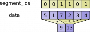
https://www.tensorflow.org/api_docs/python/math_ops/segmentation
What is also not mentioned is the behavior when using a multi-dimensional vector for data. This is exactly what happens in SyntaxNet. But, it turns out that each index of each subelement is just summed.
Because we have one unique index per feature id in all of our feature groups, unsorted_segment_sum() effectively does nothing at all and just returns the original embeddings array. That’s mainly because I don’t know how to construct an example to get multiple ids per index. (Sorry for the anticlimax). But, if we did have multiple ids, their embeddings would simply be summed for each index. Just imagine that the multiple indices 0, 0, and 0 in the example diagram are different feature ids for one index. And imagine their embeddings are 5,1,3 like in the example. Then, this feature group would end up using their sum, 9, as the embedding.
Glossary
tag: a POS tag (but it could also include POS category depending on the task context settings, apparently)
label: used interchangeably with DEPREL to define a dependency relation
arc: a label as it is made in the dependency tree (really defines a relation between two elements in the non-projective tree). This is part of the arc-standard dependency parser
action: an integer encoding of possible transitions {SHIFT, LEFT_ARC(T), RIGHT_ARC(T)} for each deprel label T
state: a state of the arc standard parser including current token number, all HEADS, all LABELS, etc…
feature type: it’s just one feature listed in context.pbtxt, such as input.tag
feature extractor: an extractor that extracts all features in a feature group for a particular parser state (contains one feature function per feature in the group)
feature function: a way to evaluate the eventual integer or floating point encoding value for a particular feature
Here is the original version (with some extra unorganized goodies at the end):
https://docs.google.com/document/d/1dPMkyzh7-QeSk7ONUuMTj9lY6flQ0NXdWcYzcMtG2oc/edit?usp=sharing